This paper is joint work with Ryan Murray. You can view the paper via the link above.
A web version of the paper is given below.
Abstract
We study metastability in the transformer attention dynamics of (Geshkovski et al., 2025), where $n$ tokens evolve as interacting particles on $S^{d-1}$. While prior work focuses on eventual collapse to a single consensus point, we observe that the dynamics consistently pass first through a prolonged bipodal phase that dominates the total evolution time. For $Q = V = I$, $\beta = 1$, $K = \mathrm{diag}(a,b)$ on $S^1$, linearization around the two-cluster equilibrium yields a single positive Jacobian eigenvalue $e^{-\gamma}$, where $\gamma(\phi) = a\cos^2\phi + b\sin^2\phi$, making the bipodal state an unstable saddle with exponentially slow escape; the clusters preferentially align with the dominant axis of $K$. Numerically, the convergence time satisfies $T(n) \approx C(a,b)\ln n + D(a,b)$, where $C$ grows exponentially in $\gamma^{\ast} = \max(a,b)$ and increases with anisotropy $b-a$. The same three-phase behavior persists on $S^2$.
Introduction
The mathematical study of transformer architectures (Vaswani et al., 2023) has attracted growing interest, motivated in part by the observation that the discrete layer-by-layer processing of tokens can be recast as a continuous-time dynamical system. Following the perspective put forward for residual networks (E, 2017) (Chen et al., 2019), one views the successive layers as time discretizations of a continuous dynamical system of interacting particles. Layer normalization constrains each token to the unit sphere $S^{d-1}$, while the self-attention mechanism provides a nonlinear coupling between tokens. Together, these give rise to the following interacting particle system, studied in detail by (Geshkovski et al., 2025): $n$ particles $x_1(t),\ldots,x_n(t)$ on $S^{d-1} \subset \mathbb{R}^d$ evolve as
\[\dot{x}_i(t) = P^{\perp}_{x_i(t)}\!\left( \frac{1}{Z_i(t)} \sum_{j=1}^{n} e^{\beta \langle Q x_i, K x_j\rangle} V x_j \right), \tag{1}\]where $P^{\perp}_x y = y - \langle x, y\rangle x$ is the tangent-space projection and $Z_i$ is a normalization constant.
Under mild assumptions, all particles eventually collapse to a single consensus point, and most existing work focuses on this terminal behavior. In this writeup, we draw attention instead to the intermediate dynamics. In every numerical experiment we have run, the system rapidly forms two nearly antipodal clusters within a few hundred Euler steps, then remains in this bipodal configuration for orders of magnitude longer before the final collapse occurs. This metastable state dominates the dynamics. The system spends the vast majority of its total evolution in the two-cluster regime. Notably, the initial clustering (Phase I) completes within a few hundred Euler steps, suggesting that in transformer architectures of realistic depth, tokens may generically form two clusters before the dynamics fully converge, consistent with the clustering behavior predicted theoretically in (Geshkovski et al., 2025).
Our analytical results are specific to $d = 2$. We restrict to the simplified setting $Q = V = I$, $\beta = 1$, and $K = \mathrm{diag}(a,b)$ with $d = 2$, in which the dynamics reduce to a system of angular ODEs on $S^1$, and we show through linearization that the bipodal states are unstable equilibria. The higher-dimensional case $d \geq 3$ is studied numerically in Numerical Dynamics on $S^2$.
Setup and Reduction to Angular Dynamics
We work with $n$ points on $S^1 \subset \mathbb{R}^2$, parametrized by angles $\theta_i(t)$ so that $x_i(t) = (\cos\theta_i(t), \sin\theta_i(t))$. Setting $Q = V = I$, $\beta = 1$, and using the uniformly normalized model ($Z_i = n$), the dynamics (1) reduce to (see Appendix A for the derivation):
\[\dot{\theta}_i(t) = -\frac{1}{n}\sum_{j=1}^{n} e^{w_{ij}(t)} \sin(\theta_i(t) - \theta_j(t)), \tag{2}\]where
\[w_{ij} = \frac{a+b}{2}\cos(\theta_i - \theta_j) + \frac{a-b}{2}\cos(\theta_i + \theta_j).\]Remark. When $K = 0$, we have $w_{ij} = 0$ and the dynamics (2) reduce to the classical Kuramoto model (Kuramoto, 1975) with zero natural frequencies and uniform coupling (see Appendix B for derivation).
The Three Phases of Evolution
Numerical experiments reveal a consistent three-phase pattern:
-
Phase I — Rapid clustering. Starting from random initial conditions, the particles quickly sort themselves into two clusters on roughly opposite sides of the circle.
-
Phase II — Metastable plateau. The two clusters sit nearly antipodally and evolve extremely slowly. The speed $|\dot{x}_i|$ drops by several orders of magnitude. This phase dominates the total evolution time.
-
Phase III — Final collapse. One cluster eventually overtakes the other, and all particles rapidly merge into a single consensus point.
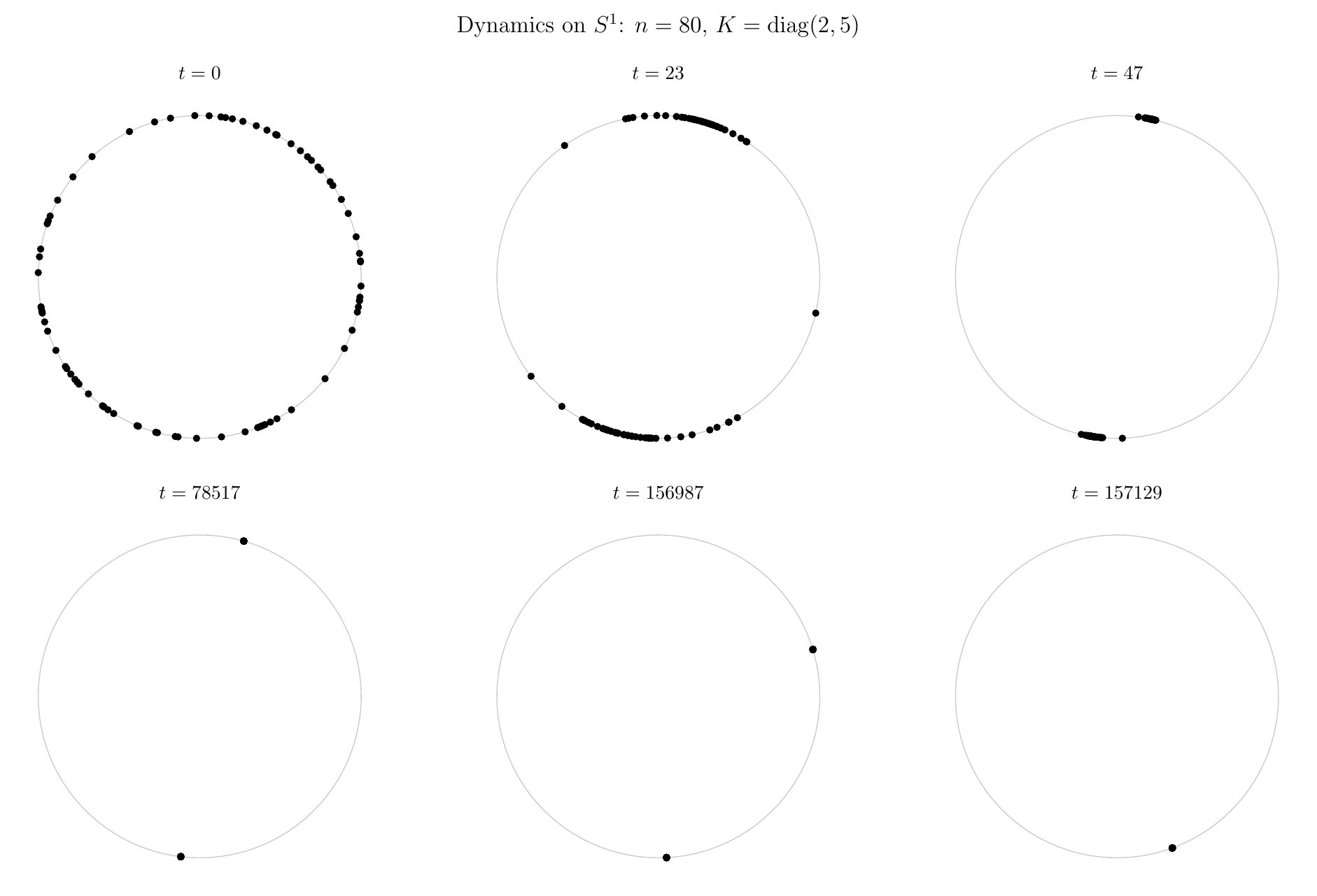
The figure below shows the geometry at representative snapshots. The initial random cloud quickly condenses into two tight clusters on opposite sides of the circle (Phase I), these clusters then sit nearly frozen for a long period (Phase II), before one absorbs the other in a rapid final merger (Phase III).
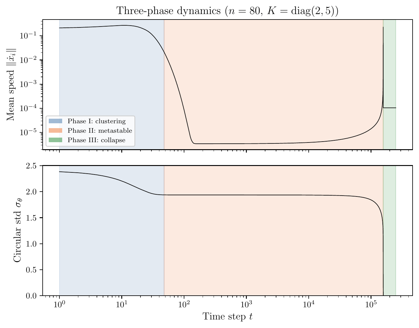
The following figure makes the time-scale separation quantitative, showing that the mean particle speed drops by roughly three orders of magnitude at the Phase I–II transition and remains depressed throughout the plateau, confirming that Phase II truly dominates the total evolution time.
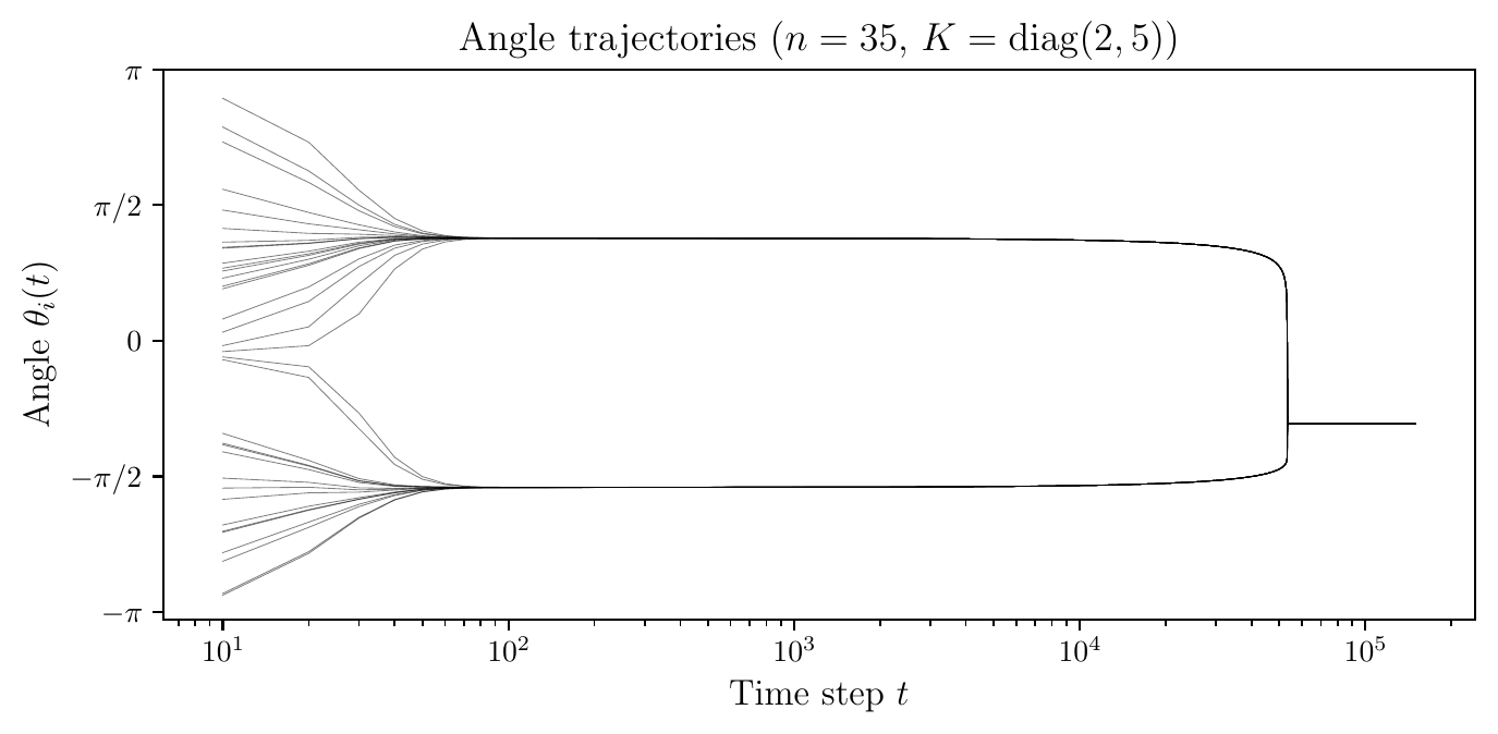
The next figure reveals the preferred orientation where the two clusters settle near $\theta \approx \pm\pi/2$, aligned with the axis corresponding to the larger diagonal entry $b = 5$ of $K$. This preferential alignment follows from the theory in Linearized Analysis of the Bipodal State, where the metastable lifetime is longest when the bipodal configuration maximizes $\gamma(\phi)$, which for $b > a$ occurs at $\phi = \pi/2$.
Linearized Analysis of the Bipodal State
To understand the metastable behavior analytically, we linearize the dynamics (2) about the two-cluster equilibrium.
Consider a perfectly bipodal configuration at angle $\phi$:
\[\theta = (\underbrace{\phi, \ldots, \phi}_{n/2},\ \underbrace{\phi + \pi, \ldots, \phi + \pi}_{n/2}).\]Define
\[\gamma(\phi) := a\cos^2\phi + b\sin^2\phi, \tag{3}\]which interpolates between $\gamma(0) = a$ and $\gamma(\pi/2) = b$. A direct computation of the Jacobian at this configuration yields the eigenvalues (see Appendix C for the full derivation):
\[\lambda_1 = 0, \qquad \lambda_2 = \cdots = \lambda_{n-1} = -\sinh(\gamma), \qquad \lambda_n = e^{-\gamma} > 0. \tag{4}\]The eigenvalue structure (4) has a direct dynamical interpretation. The zero eigenvalue $\lambda_1 = 0$ reflects mean-angle conservation; the bipodal state sits in a one-parameter family parametrized by $\phi$. The $n-2$ negative eigenvalues $-\sinh(\gamma)$ enforce within-cluster cohesion once approximate clusters form, completing Phase I. The single positive eigenvalue $\lambda_n = e^{-\gamma}$ controls the escape rate from the bipodal saddle: since $\gamma(\phi) = a\cos^2\phi + b\sin^2\phi \in [\min(a,b),\,\max(a,b)]$, the value of $\gamma$ is fixed once $a$ and $b$ are chosen, and grows only as $a$ and $b$ grow. When $a$ and $b$ are large, $e^{-\gamma}$ is exponentially small, making escape from the saddle extremely slow and the metastable lifetime exponentially long.
Since the unstable eigenvalue is $e^{-\gamma(\phi)}$, the most metastable bipodal state (slowest escape) occurs at the orientation $\phi^{\ast}$ that maximizes $\gamma(\phi) = a\cos^2\phi + b\sin^2\phi$. If $a > b$, then $\phi^{\ast} = 0$ (clusters along the $e_1$-axis); if $b > a$, then $\phi^{\ast} = \pi/2$ (clusters along the $e_2$-axis). In either case, the system preferentially gets trapped along the dominant axis of $K$. With $K = \mathrm{diag}(2,5)$, we have $b > a$, and the two clusters consistently settle near $\theta \approx \pm\pi/2$, the $e_2$-axis. The same effect governs the $S^2$ experiments of Numerical Dynamics on $S^2$, where the dominant axis is the $z$-axis.
Additionally, we also note two propositions about the dynamics:
Proposition 1 (Mean conservation). The arithmetic mean angle $\bar{\theta}(t) = \frac{1}{n}\sum_i \theta_i(t)$ is conserved: $\dot{\bar{\theta}} = 0$.
Proof. Since $w_{ij} = w_{ji}$ and $\sin(\theta_i - \theta_j) = -\sin(\theta_j - \theta_i)$, the double sum $\sum_i \sum_j e^{w_{ij}}\sin(\theta_i - \theta_j)$ vanishes by antisymmetry. $\square$
Proposition 2 (Unique semicircular equilibrium). If $\theta^{\ast}$ is an equilibrium with all angles contained in an open semicircle (i.e., $\max_i \theta_i^{\ast} - \min_i \theta_i^{\ast} < \pi$), then $\theta_1^{\ast} = \cdots = \theta_n^{\ast}$.
Proof. Let $m = \arg\max_k \theta_k^{\ast}$. At equilibrium, $0 = \dot\theta_m^{\ast} = f_m(\theta^{\ast})$, which means $0 = \sum_{j=1}^{n} e^{w_{mj}}\sin(\theta_m^{\ast} - \theta_j^{\ast})$. Since $\max_i\theta_i^{\ast} - \min_i\theta_i^{\ast} < \pi$, each term satisfies $\sin(\theta_m^{\ast} - \theta_j^{\ast}) \geq 0$ with $e^{w_{mj}} > 0$. A sum of non-negative terms can only be zero if every term is zero, i.e., $\sin(\theta_m^{\ast} - \theta_j^{\ast}) = 0$ for all $j$. Since $\lvert\theta_m^{\ast} - \theta_j^{\ast}\rvert < \pi$, this forces $\theta_j^{\ast} = \theta_m^{\ast}$ for all $j$. $\square$
These results rule out non-consensus equilibria confined to a semicircle, leaving bipodal states as the only non-trivial equilibria observed numerically.
Scaling Laws
The eigenvalue analysis of Linearized Analysis of the Bipodal State suggests that the duration of the metastable plateau grows exponentially in $\gamma$. To quantify the dependence on $n$ we record $T$, the number of Euler steps until $\sigma_\theta < 0.05$ (Euler step $h = 0.1$), sweeping 30 log-spaced values of $n$ per configuration. For the isotropic case $K = aI$ we sweep $n$ from $5$ to $3000$ with 20 seeds per point, testing $a \in {1.0, 1.5, 2.0, 2.5, 3.0, 3.5, 4.0, 4.5, 5.0}$. For anisotropic $K = \mathrm{diag}(a,b)$ with $a \neq b$, we test seven $\gamma^{\ast}$-levels spanning ${2.0, 2.5, 3.0, 3.5, 4.0, 4.5, 5.0}$, using one or two distinct $(a,b)$ pairs per level; the $n$-range and number of seeds per pair are scaled down for larger $\gamma^{\ast}$ to account for the exponential growth of run-time.
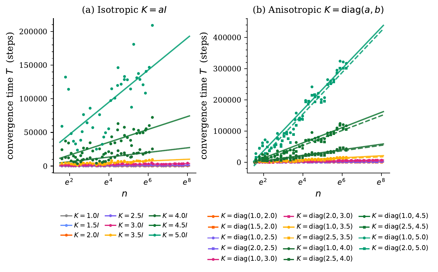
The figures below show that both isotropic and anisotropic $K$ follow the same logarithmic scaling law; however, the key difference is that anisotropic pairs have substantially larger prefactors $C$ than the isotropic case at the same $\gamma^{\ast}$.
For an anisotropic $K = \mathrm{diag}(a,b)$, $a \neq b$, the convergence time follows a logarithmic law,
\[T(n) \;\approx\; C(K)\,\ln n + D(K), \tag{5}\]with fitted slope $C(K)$ that grows exponentially in $\gamma^{\ast} = \max(a,b)$. However, $C$ is not determined by $\gamma^{\ast}$ alone; at fixed $\gamma^{\ast}$, pairs with smaller anisotropy $b - a$ produce a smaller fitted slope.
The isotropic case, with $K = aI$, also obeys $T(n) \approx C(a,a)\,\ln n + D(a,a)$, but with a substantially smaller prefactor than any anisotropic pair sharing the same $\gamma^{\ast} = a$. For small $a$ (e.g. $a \leq 2$) this makes the isotropic curves appear nearly flat over the range $n \in [100, 3000]$; for large $a$ (e.g. $a \geq 3.5$) the logarithmic growth is visible even in isotropic data. The isotropic entry therefore represents the $b = a$ case of the general prefactor $C(a,b)$, and forms the lower boundary at each $\gamma^{\ast}$ level. One possible explanation stems from the behavior of $\gamma(\phi)$ in the two cases. For isotropic $K = aI$, we have $\gamma(\phi) = a$ for all $\phi$: the barrier height is the same in every direction, so all bipodal orientations are equally metastable and no axis is preferred by $K$. The two clusters that form in Phase I therefore settle along a direction determined by the initial conditions rather than by $K$, and they land at a typical distance from the saddle. For anisotropic $K$, $\gamma(\phi)$ varies with $\phi$, and Phase I drives the clusters toward the most metastable orientation $\phi^{\ast}$ (the dominant axis of $K$), leaving them unusually close to the saddle and producing the larger prefactor $C$.
| $K$ | $b - a$ | $\gamma^{\ast}$ | $C(K)$ (fitted) |
|---|---|---|---|
| $\mathrm{diag}(1.5,1.5)$ | $0$ | $1.5$ | $16.8$ |
| $\mathrm{diag}(2,2)$ | $0$ | $2.0$ | $43.2$ |
| $\mathrm{diag}(1,2)$ | $1.0$ | $2.0$ | $135$ |
| $\mathrm{diag}(2.5,2.5)$ | $0$ | $2.5$ | $132$ |
| $\mathrm{diag}(3,3)$ | $0$ | $3.0$ | $405$ |
| $\mathrm{diag}(1,3)$ | $2.0$ | $3.0$ | $1{,}080$ |
| $\mathrm{diag}(5,5)$ | $0$ | $5.0$ | $23{,}885$ |
| $\mathrm{diag}(2,5)$ | $3.0$ | $5.0$ | $66{,}615$ |
The figure below plots the fitted slope $C$ against $\gamma^{\ast}$ for every simulated $K$. The anisotropic entries (diamonds) grow exponentially in $\gamma^{\ast}$, but at each fixed $\gamma^{\ast}$ the slope varies across pairs, with smaller anisotropy $b - a$ yielding a smaller $C$. The isotropic entries (circles) form the lower boundary at each $\gamma^{\ast}$, the $b = a$ case of the general prefactor $C(a,b)$.

Numerical Dynamics on $S^2$
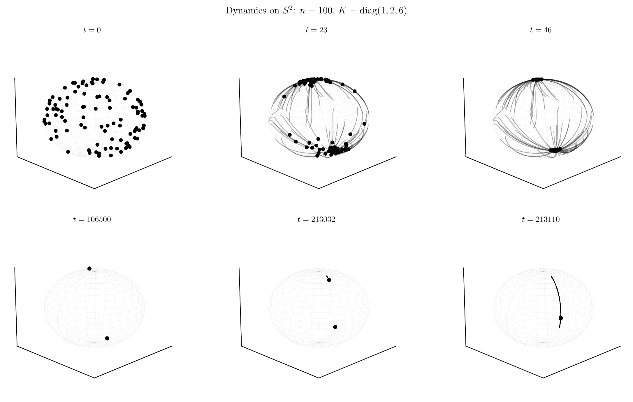
The metastable phenomenon is not limited to the circle; we present here numerical evidence that it persists in $d = 3$, though an analytical treatment analogous to Linearized Analysis of the Bipodal State remains open. The figure below shows the dynamics of $n = 100$ particles on $S^2 \subset \mathbb{R}^3$ with $K = \mathrm{diag}(1, 2, 6)$. The same three-phase pattern is visible, with a rapid initial sorting into two antipodal clusters (Phase I), a prolonged plateau during which the clusters are nearly stationary (Phase II), and a final collapse to a single consensus point (Phase III).
The dominant axis of $K$ is the $z$-axis (eigenvalue $6$), and the metastable clusters settle near the north and south poles, consistent with the orientation theory of Linearized Analysis of the Bipodal State.
Discussion & Open Problems
The linearization reveals that the bipodal state has one small unstable direction, and the system takes a long time to find it. Simulations confirm that the escape time follows $T(n) \approx C(K)\ln n + D(K)$ for all tested $K$, with the prefactor $C$ growing exponentially in $\gamma^{\ast}$ and increasing with the anisotropy gap $b-a$. We close with four open problems.
Conjecture 1 (Logarithmic scaling law). For $K = \mathrm{diag}(a,b)$ with $a \neq b$ and random initial conditions, the escape time satisfies
\[T(n) \;=\; C(a,b)\,\ln n + D(a,b) \qquad \text{as } n \to \infty,\]where $C(a,b)$ grows exponentially in $\gamma^{\ast} = \max(a,b)$ and increases with $b - a$. The isotropic case $b = a$ follows the same law with $C(a,a)$ the smallest value at fixed $\gamma^{\ast} = a$.
The logarithmic law holds across all simulated pairs. A rigorous proof remains open.
Conjecture 2 (Bipodal equilibrium structure). For $K = \mathrm{diag}(a,b)$ with $a, b > 0$, the only steady states of (2) are the consensus states (all tokens equal) and the bipodal states (tokens split into two antipodal groups). No three-or-more-cluster steady states exist.
Proposition 2 rules out non-consensus steady states on any open semicircle, and no others have been observed numerically.
Conjecture 3 (Universality of the three-phase pattern). For generic starting configurations on $S^{d-1}$, the dynamics always pass through the same three phases: rapid clustering into two groups (Phase I), a prolonged bipodal plateau (Phase II), and a final collapse to a single consensus point (Phase III).
All experiments here use uniformly random initial conditions. Whether the three-phase pattern persists for structured or adversarially chosen initial data remains open.
Conjecture 4 (Lyapunov structure). There is an energy function $E\colon (S^1)^n \to \mathbb{R}$ for the dynamics (2) such that bipodal states are saddle points of $E$ and consensus states are local minima.
The Kuramoto model ($K = 0$) has a known energy function; finding one for $K \neq 0$ remains open.
Appendix A: Derivation of the Angular ODE
We show the reduction from (1) to (2) under the assumptions $Q = V = I$, $\beta = 1$, $K = \mathrm{diag}(a,b)$, and $Z_i = n$ (uniformly normalized model). Each particle lives on $S^1$, so we write
\[x_i(t) = \cos(\theta_i(t))\, e_1 + \sin(\theta_i(t))\, e_2.\]We first compute $\langle x_i, Kx_j \rangle$. Since $K = \mathrm{diag}(a,b)$, we have
\[\langle x_i, Kx_j \rangle = a\cos\theta_i\cos\theta_j + b\sin\theta_i\sin\theta_j = \frac{a+b}{2}\cos(\theta_i - \theta_j) + \frac{a-b}{2}\cos(\theta_i + \theta_j),\]where the second equality follows from the product-to-sum identities. We denote this quantity $w_{ij}$, so that $\langle x_i, Kx_j \rangle = w_{ij}$. To extract an ODE for $\theta_i$, we differentiate the identity $\cos(\theta_i(t)) = \langle x_i(t), e_1 \rangle$ with respect to $t$, giving
\[-\sin(\theta_i)\,\dot{\theta}_i = \langle \dot{x}_i, e_1 \rangle.\]Substituting the dynamics \(\dot{x}_i = P^{\perp}_{x_i}\!\bigl(\frac{1}{n}\sum_j e^{w_{ij}} x_j\bigr)\) and using \(\langle P^{\perp}_{x_i} v, e_1 \rangle = \langle v, e_1 \rangle - \langle v, x_i \rangle\cos\theta_i\) yields
\[-\sin(\theta_i)\,\dot{\theta}_i = \frac{1}{n}\sum_{j=1}^{n} e^{w_{ij}}\Bigl[\langle x_j, e_1\rangle - \langle x_j, x_i\rangle\cos\theta_i\Bigr].\]Substituting $\langle x_j, e_1 \rangle = \cos\theta_j$ and $\langle x_j, x_i \rangle = \cos(\theta_i - \theta_j)$ and dividing by $-\sin(\theta_i)$, the bracket becomes
\[\frac{\cos\theta_j - \cos(\theta_i - \theta_j)\cos\theta_i}{\sin\theta_i} = \sin(\theta_i - \theta_j),\]where the last step is a standard trigonometric identity (expanding $\cos(\theta_i - \theta_j) = \cos\theta_i\cos\theta_j + \sin\theta_i\sin\theta_j$ and simplifying). This gives (2).
Appendix B: Derivation of the Kuramoto Model
We show that when $K = 0$ the dynamics (2) reduce to the Kuramoto model with zero natural frequencies. Setting $K = 0$ means $w_{ij} = 0$ for all $i,j$, so (2) becomes
\[\dot{\theta}_i(t) = -\frac{1}{n}\sum_{j=1}^{n}\sin(\theta_i(t) - \theta_j(t)) = \frac{1}{n}\sum_{j=1}^{n}\sin(\theta_j(t) - \theta_i(t)),\]which is exactly the Kuramoto model
\[\dot{\theta}_i(t) = \omega_i + \frac{\kappa}{n}\sum_{j=1}^{n}\sin(\theta_j(t) - \theta_i(t))\]with natural frequencies $\omega_i = 0$ and coupling strength $\kappa = 1$.
Appendix C: Derivation of the Eigenvalues
We derive the eigenvalues (4) of the Jacobian $A = D_\theta f$ of the vector field $f_i(\theta) = -\frac{1}{n}\sum_j e^{w_{ij}}\sin(\theta_i - \theta_j)$, evaluated at the general bipodal state
\[\theta^{\ast} = (\underbrace{\phi, \ldots, \phi}_{n/2},\; \underbrace{\phi+\pi, \ldots, \phi+\pi}_{n/2}).\]To compute the Jacobian, we introduce the shorthand $s_{ij} = \sin(\theta_i - \theta_j)$ and $c_{ij} = \cos(\theta_i - \theta_j)$. Differentiating $f_i$ with respect to $\theta_k$ requires the partial derivatives of both $s_{ij}$ and $w_{ij}$. For $s_{ij}$, we have
\[\frac{\partial s_{ij}}{\partial \theta_k} = c_{ij}(\delta_{ik} - \delta_{jk}).\]For $w_{ij} = \frac{a+b}{2}\cos(\theta_i - \theta_j) + \frac{a-b}{2}\cos(\theta_i + \theta_j)$, differentiating gives
\[\frac{\partial w_{ij}}{\partial \theta_i} = -\frac{a+b}{2}s_{ij} - \frac{a-b}{2}\sin(\theta_i + \theta_j), \qquad \frac{\partial w_{ij}}{\partial \theta_j} = \frac{a+b}{2}s_{ij} - \frac{a-b}{2}\sin(\theta_i + \theta_j),\]and $\frac{\partial w_{ij}}{\partial \theta_k} = 0$ for $k \notin {i,j}$. Substituting into the product-rule expansion of $\frac{\partial f_i}{\partial \theta_k}$ and separating the diagonal ($k = i$) and off-diagonal ($k \neq i$) cases yields
\[\begin{aligned} A_{ii} &= -\frac{1}{n}\sum_{j \neq i} e^{w_{ij}} \Bigl[\frac{\partial w_{ij}}{\partial \theta_i} s_{ij} + c_{ij}\Bigr], \\[6pt] A_{ik} &= -\frac{1}{n}\, e^{w_{ik}} \Bigl[\frac{\partial w_{ik}}{\partial \theta_k} s_{ik} - c_{ik}\Bigr] \quad (k \neq i). \end{aligned}\]Now we evaluate at $\theta^{\ast}$. The key observation is that $\theta_i - \theta_j$ is always either $0$ (within the same cluster) or $\pm\pi$ (across clusters), so $s_{ij} = \sin(\theta_i - \theta_j) = 0$ for every pair. Since every term involving $s_{ij}$ vanishes, the Jacobian entries simplify dramatically to
\[A_{ii} = -\frac{1}{n}\sum_{j \neq i} e^{w_{ij}} c_{ij}, \qquad A_{ik} = \frac{1}{n} e^{w_{ik}} c_{ik} \quad (k \neq i).\]It remains to evaluate $w_{ij}$ and $c_{ij}$. Recalling $\gamma = \gamma(\phi) = a\cos^2\phi + b\sin^2\phi$, a direct substitution gives:
- Within the same cluster ($\theta_i - \theta_j = 0$, $\theta_i + \theta_j = 2\phi$): $c_{ij} = 1$ and $w_{ij} = \gamma$.
- Across clusters ($\theta_i - \theta_j = \pm\pi$, $\theta_i + \theta_j = 2\phi \pm \pi$): $c_{ij} = -1$ and $w_{ij} = -\gamma$.
Setting $\mu = \frac{1}{n}e^{\gamma}$ and $\nu = \frac{1}{n}e^{-\gamma}$, each within-cluster off-diagonal entry equals $\mu$ and each cross-cluster off-diagonal entry equals $-\nu$. The diagonal entry for particle $i$ sums over $\frac{n}{2}-1$ within-cluster neighbors and $\frac{n}{2}$ cross-cluster neighbors:
\[A_{ii} = -\!\left(\tfrac{n}{2}-1\right)\mu + \tfrac{n}{2}\nu.\]Label the clusters $X$ (indices $1,\ldots,n/2$) and $Y$ (indices $n/2+1,\ldots,n$). The full Jacobian has the block form
\[A = \begin{bmatrix} A_{XX} & A_{XY} \\ A_{YX} & A_{YY} \end{bmatrix},\]where $A_{XX} = A_{YY}$ has diagonal $-(\frac{n}{2}-1)\mu + \frac{n}{2}\nu$ and off-diagonal $\mu$, while $A_{XY} = A_{YX}$ is the $\frac{n}{2}\times\frac{n}{2}$ constant matrix with every entry equal to $-\nu$. This can be written as
\[A = \underbrace{\left(-\tfrac{n}{2}\mu + \tfrac{n}{2}\nu\right)}_{= -\sinh\gamma} I + C,\]where $C$ has blocks $\mu\,\mathbf{1}\mathbf{1}^\top$ on the diagonal and $-\nu\,\mathbf{1}\mathbf{1}^\top$ off the diagonal, with $\mathbf{1}$ denoting the all-ones vector of length $n/2$. Since the scalar shift $-\sinh(\gamma)$ moves all eigenvalues uniformly, we only need to find the eigenvalues of $C$.
$C$ is a rank-2 matrix. To see this, note that its column space is spanned by just two vectors: $v_+ = (\mathbf{1}, \mathbf{1}) \in \mathbb{R}^n$ and $v_- = (\mathbf{1}, -\mathbf{1}) \in \mathbb{R}^n$. A direct computation gives
\[Cv_+ = \tfrac{n}{2}(\mu - \nu)\,v_+, \qquad Cv_- = \tfrac{n}{2}(\mu + \nu)\,v_-.\]So $v_+$ and $v_-$ are eigenvectors of $C$ with eigenvalues
\[\frac{n}{2}(\mu - \nu) = \frac{e^\gamma - e^{-\gamma}}{2} = \sinh(\gamma), \qquad \frac{n}{2}(\mu + \nu) = \frac{e^\gamma + e^{-\gamma}}{2} = \cosh(\gamma),\]respectively, and all other $n-2$ eigenvalues of $C$ are $0$.
Adding back the scalar shift $-\sinh(\gamma)$ from the identity term, the eigenvalues of $A$ are:
\[\begin{aligned} &-\sinh(\gamma) + \sinh(\gamma) = 0 &&\text{(multiplicity 1, eigenvector } v_+\text{),} \\ &-\sinh(\gamma) + 0 = -\sinh(\gamma) &&\text{(multiplicity } n-2\text{),} \\ &-\sinh(\gamma) + \cosh(\gamma) = e^{-\gamma} > 0 &&\text{(multiplicity 1, eigenvector } v_-\text{),} \end{aligned}\]which is precisely (4). $\blacksquare$
References
- Geshkovski, B., Letrouit, C., Polyanskiy, Y., & Rigollet, P. (2025). A mathematical perspective on Transformers. https://arxiv.org/abs/2312.10794
- Vaswani, A., Shazeer, N., Parmar, N., Uszkoreit, J., Jones, L., Gomez, A. N., Kaiser, L., & Polosukhin, I. (2023). Attention Is All You Need. https://arxiv.org/abs/1706.03762
- E, W. (2017). A Proposal on Machine Learning via Dynamical Systems. Communications in Mathematics and Statistics, 5(1), 1–11. https://doi.org/10.1007/s40304-017-0103-z
- Chen, R. T. Q., Rubanova, Y., Bettencourt, J., & Duvenaud, D. (2019). Neural Ordinary Differential Equations. https://arxiv.org/abs/1806.07366
- Kuramoto, Y. (1975). Self-entrainment of a population of coupled non-linear oscillators. Lect. Notes Phys., 39, 420–422. https://doi.org/10.1007/BFb0013365